Kien van Ho · Portfolio

Kien van Ho

Engineer combining physics-based modelling, machine learning and energy systems

I build models that keep the physics and learn from the data, and I test them on small, expensive datasets from gas turbines, robots and engines. The aim is life, energy and efficiency predictions that stay physically plausible.

I size, balance and model energy and process systems: parked EV fleets as grid storage, a drinking-water plant, CHP and Power-to-Gas cases. In industry I planned production for an electric-motor line and modelled energy use on the shop floor.

Degree
Erasmus Mundus double M.Sc. (ME3+)
Industry
Siemens Energy · Mercedes-Benz
Based in
Berlin

Open to entry-level roles in ML, data science and hybrid modelling for the energy transition.

Open to entry-level roles in energy-systems and process engineering for the energy transition.

Explore work

Project index · ML & modelling

    ML & modelling

    Selected work

    The projects with the strongest evidence for this view. Each card states the problem, my part, the result and its main limit; the case study underneath has the method and validation.

    Type
    Master's thesis
    Partner
    Siemens Energy
    Period
    Feb – Aug 2026
    Team
    Individual

    Gas turbines · fracture mechanics · hybrid ML

    Physics-informed ML for short-crack growth

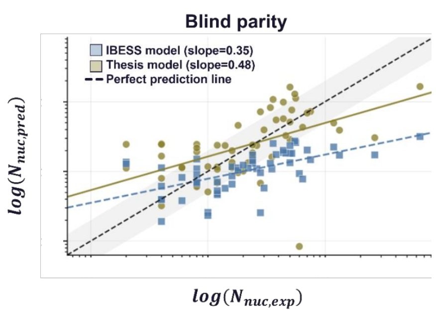
    A neural network that predicts crack-growth curves for gas-turbine components with manufacturing defects, trained on experiments and held to the shape of an established fracture-mechanics model (IBESS) through its loss.
    Problem
    The physical short-crack model is interpretable but systematically underestimated fatigue life on the experiments; with 56 specimens a free black-box model would overfit.
    My part
    Individual thesis in the Predictive Analytics team at Siemens Energy: model design, physics loss, nested cross-validation and all implementation.
    Result
    −20.1% mean absolute log error vs. the physics baseline (0.965 → 0.771), each of the 56 specimens predicted blind.
    Limit
    29 of 56 predictions now overestimate life (baseline: 8), the unsafe direction. A feasibility study, not a certified lifetime assessment.
    PythonTensorFlowscikit-learnpandasNested CVCustom physics lossMethod code, synthetic data ↗
    Blind parity plot of predicted versus experimental cycles to nucleation on log axes. Thesis model points (slope 0.48) sit closer to the perfect-prediction line than baseline points (slope 0.35).
    Blind predictions vs. experiment, cycles to crack nucleation. Squares: physical baseline (IBESS). Circles: thesis model. Axis values hidden.
    Full case study: model design, validation, limits

    Starting point

    The physical short-crack model (IBESS) is interpretable but, on the experimental data, it systematically underestimated fatigue life. With only 56 specimens from one material at one nominal stress ratio (R = 0.1), a free black-box model would overfit and lose physical meaning.

    What the network predicts

    Instead of free values at every point, the network outputs 16 decoder parameters per specimen: 7 density knots each for the depth and surface crack fronts, one terminal surface-to-depth ratio, and one cycle "warp" multiplier. Integrating and normalising the knots guarantees monotonically growing crack curves by construction.

    Inputs

    Initial defect size (a₀, c₀), max/min stress, specimen width and thickness, defect type (surface or embedded, one-hot), plus derived aspect ratio, stress range, stress ratio (nominally 0.1 throughout, so it carries little information) and log-transformed size and load terms. All standardised. The physics curves are not network inputs: they supervise the curve shape through the loss, and the physics model's threshold cycle sets the time scale that the warp multiplier corrects.

    Loss function

    Total loss = experimental error (MSE of log cycles) + four physics penalties: curve shape vs. IBESS, terminal crack-front ratio, concavity of the threshold curve (checked at 17 points), and a cap on the warp correction so timing cannot absorb all the error.
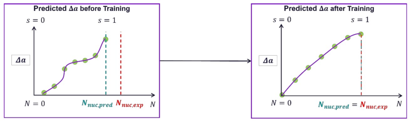
    Two panels: before training, the predicted crack-extension curve through seven green density knots is irregular and the predicted nucleation cycle misses the experimental one; after training the curve is smooth and both cycle markers coincide.
    Schematic: seven density knots (green) shape the predicted crack-extension curve, and training aligns predicted and experimental nucleation cycles.

    Validation

    • Nested cross-validation with 5 outer folds, so each of the 56 specimens gets exactly one blind prediction.
    • Loss weights tuned by repeated inner validation inside each outer training fold.
    • Preprocessing, feature construction and model selection all fitted inside training folds only, to rule out leakage.
    • After prediction, physical quantities (geometry, crack closure, J-integral, ΔK, da/dN) are recomputed as a consistency check.

    Results

    MetricBaselineThesisChange
    MAE (log)0.9650.771−20.1%
    RMSE (log)1.1711.062−9.3%
    Late predictions8 / 5629 / 56+21

    Errors are measured in natural-log cycle space, so the typical miss shrank from a factor of about 2.6 to about 2.2 in cycles. The error distribution moved from a consistent underestimate to centred on zero, and the median prediction ratio moved close to 1. The smaller RMSE gain shows that typical predictions improved more than the worst ones.

    Limits I documented. A "late" prediction overestimates life, which is the unsafe direction, so the model is less conservative than the baseline. One specimen was predicted at more than three times its measured life, showing instability with so little data. A deployable version would need a lower bound, a one-sided loss or a safety factor, and data across more materials and stress ratios. The thesis is a feasibility study, not a certified lifetime assessment.
    Public code (2026). The repository re-implements the method on synthetic specimens (the experiments and the partner's physics code are private, and nothing in it reproduces the numbers above). It benchmarks the decoder against simpler corrections of the same physics model on identical cross-validation folds. On that synthetic task a 15-parameter ridge regression on the log lifetime correction beats the 1,280-parameter decoder (MAE in log cycles 0.265 vs. 0.314 over three fold seeds), while the decoder leaves fewer late predictions (26 vs. 31 of 56). The physics penalties change the curve shapes but barely move the lifetime error, because the lifetime is one scalar warp. I kept this negative result; the repository is a method demonstration, not evidence that the architecture is the best lifetime predictor. It also fixes a NaN gradient in the interpolation, refuses to score runs with invalid predictions, and ships a pinned environment, run manifests and CI.
    Type
    Master's project
    Context
    IMT Atlantique · GreenTwins
    Period
    Feb – Jun 2025
    Team
    Team of 3 · lead

    Digital twin · dual-fuel engine · ML services

    Digital twin of a dual-fuel engine

    A prototype twin of a 14.4 kWe dual-fuel (diesel and biogas) generator set: set power and fuel mix, and ML models plus physics formulas predict efficiency, exhaust temperature and fuel and CO₂ flows, served through an API into a 3D platform.
    Problem
    GreenTwins wanted a working twin of the lab engine: predictions for any power and fuel mix, delivered into their digital-twin platform.
    My part
    Led the team of three and did most of the implementation: ML models, energy balance, flow control and the FastAPI service.
    Result
    kNN efficiency model R² 0.93 on a random 20% hold-out; models served through FastAPI in Docker to the GreenTwins platform, code and data on Azure.
    Limit
    Prototype: inputs set by hand, no live connection to the engine. The exhaust-temperature R² is a training fit, not a held-out score. The public code runs on a synthetic engine map, not the lab data.
    Pythonscikit-learnFastAPIDockerAzureBlenderService code, synthetic engine map ↗
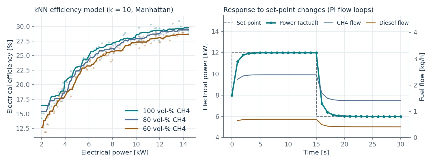
    Left: kNN electrical efficiency against power for three methane shares on a synthetic engine map. Right: power, methane flow and diesel flow following set-point changes under PI flow loops.
    From the public code on a synthetic engine map, not lab data: the efficiency model (left) and the flow loops following set-point changes (right).
    Full case study: architecture, models, validation

    How it works

    Models

    • Electrical efficiency: k-nearest-neighbours regression (k = 10, Manhattan distance) on power and methane share, tuned with 5-fold grid search; R² 0.929 on a 20% hold-out set.
    • Exhaust temperature: linear regression on power, refined with diesel share and methane content; R² 0.956 on the training data.
    • Features chosen from a correlation analysis of earlier lab engine-mapping runs on a Cat DE18E3 generator converted to dual-fuel.

    Plausibility check against lab data

    Operating point at about 80% loadTwin vs. measured
    Efficiencywithin 0.1 pp
    Exhaust temperaturewithin 1.5%
    Methane flowwithin 0.5%
    Diesel flowwithin 0.5%

    "Measured" is the nearest recorded lab operating point (raw lab data not published), which the models had seen in training, so this is a consistency check rather than independent validation. Fuel flows follow from the predicted efficiency through the energy balance. In simulation, the controller settles in under 5 seconds.
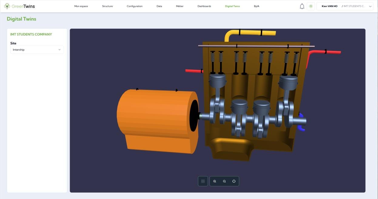
    GreenTwins platform view showing a 3D model of the engine and generator.
    Engine view inside the GreenTwins platform.
    Limits. Inputs are set by hand; a live data connection to the running engine was scoped as future work, together with controller tuning and predictive maintenance. The exhaust-temperature R² is a training fit, not a held-out score.
    Public code (2026). The repository is a simulation and inference-service prototype on a synthetic engine map; the lab data stay private, so its scores are implementation checks, not engine validation. Training is separate from serving: a command writes a versioned model bundle (models, feature schema and units, supported operating domain, data fingerprint, evaluation, dependency versions) that the service validates at startup. Requested operating points are checked against equipment limits and the training domain, including a nearest-neighbour support check, and are rejected or flagged. One simulated engine is shared by all clients on purpose, with explicit reset, stop and start semantics tested over subsequent ticks. The evaluation adds held-out operating regions and baselines: the kNN efficiency model reaches R² 0.93 on a random hold-out but cannot extrapolate into a held-out low-load band, where a ridge regression is better, and adding diesel energy share as a feature makes it worse on every split even though the synthetic generator depends on it. The exhaust-temperature R² of 0.99 is the noise floor of a linear generator and says nothing about engines.
    Type
    Internship project
    Company
    Mercedes-Benz AG
    Period
    Feb – Aug 2024
    Team
    Individual (intern)

    Hybrid modelling · industrial robots · energy efficiency

    Energy model of an assembly robot

    The physics-plus-data approach I later took further in my thesis, here on a universal robot in engine assembly: a physics-based model, a neural network that predicts its energy use, and trajectory studies to find where energy could be saved.

    Problem
    The robot's energy use depends on how it moves; the plant wanted to know how much an optimised trajectory could save.
    My part
    Individual intern project: Python physics model of the robot's energy consumption along its motion, a neural network for energy prediction validated against the robot's data, and trajectory studies.
    Result
    Up to 15% modelled energy-savings potential from optimised instead of arbitrary trajectories.
    Limit
    Modelled potential, not measured savings in production. Figures and code stay with Mercedes-Benz.
    PythonNeural networksPhysics-based modellingProduction data
    Type
    Bachelor's thesis
    Context
    TU Berlin · product development
    Period
    2024
    Team
    Individual

    Small-data regression · model selection

    Predicting vehicle attributes from early design data

    Can you predict how a car will perform from nine design parameters, with data on only 31 cars? Four regression models compared on five functional attributes.
    Problem
    Early in design, few parameters are fixed and few comparable cars exist; the question was where ML helps and where it does not.
    My part
    Individual thesis at TU Berlin: feature selection, four models (linear, Lasso, kNN, SVR), cross-validation. The work fed into a 2025 Proceedings of the Design Society paper I co-authored.
    Result
    No single model won. Passenger and cargo volume were best explained (R² up to 0.78); towing capacity was not predictable.
    Limit
    Thesis scores are optimistic (tuned and scored on the same folds). My 2026 re-check with nested, twin-aware cross-validation lowers the median R² of the four thesis models to 0.15–0.27. A plain ridge regression on all nine features does better (0.40), and the complete selection procedure, scored honestly, reaches 0.23.
    Pythonscikit-learnFeature selectionCross-validationCode and re-evaluation ↗
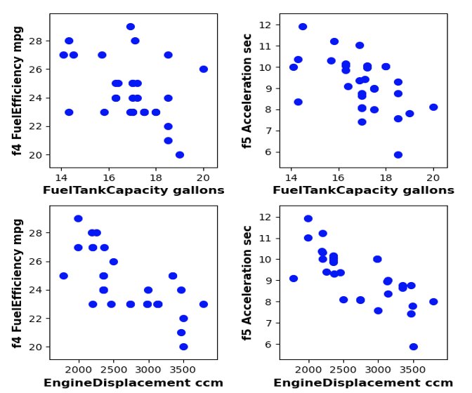
    Four scatterplots of fuel efficiency and acceleration against fuel tank capacity and engine displacement for 31 vehicles.
    Exploring the data: fuel efficiency and acceleration vs. tank capacity and engine displacement.
    Full case study: method and results

    Data and features

    31 midsize sedans sold in the US in 2002, from a published platform study (de Weck, 2006). Nine design variables: fuel tank capacity, engine displacement, front track width, wheelbase, ground clearance, height, length, tyre width and tyre diameter. One car (Honda Accord) held back as a final check.

    Method

    Mean imputation and standardisation, then sequential floating forward feature selection. Each model tuned and scored with 5-fold cross-validation, with linear regression as the literature baseline.

    Cross-validated R² by attribute, thesis protocol

    AttributeLinearLassokNNSVR
    Passenger volume0.580.590.750.78
    Cargo volume0.710.660.650.67
    Fuel efficiency0.220.160.420.15
    Acceleration0.420.350.310.38
    Towing capacity−2.91−2.830.24−0.18

    Highest per attribute highlighted. These scores are optimistic: tuning and scoring used the same folds. A later re-implementation of this protocol gives medians of 0.55–0.69 (see the 2026 re-evaluation below).

    Thesis findings

    • No single model won; the best choice depended on the attribute.
    • Passenger and cargo volume were the best explained attributes; towing capacity was not.

    Re-evaluated in 2026

    The thesis tuned and scored on the same folds, and badge-engineered twins such as the Ford Taurus and Mercury Sable could land on both sides of a split. I re-implemented that protocol (median R² 0.55–0.69 across models) and compared it with repeated nested cross-validation that keeps twins in the same fold, after dropping 11 placeholder towing values. The median R² of the four thesis models falls to 0.15–0.27. Three baselines on the same folds change the picture: a ridge regression on all nine features, with no feature selection, has the best median (0.40) and wins on passenger volume and acceleration; Lasso without feature selection matches Lasso with it. Sequential feature selection costs 80–99% of the runtime and picks a different subset in most folds, so it mainly adds instability here. Picking the "best" model family after seeing the outer scores is itself optimistic: when family, hyperparameters and features are all chosen inside the inner loop, the complete procedure scores 0.23, below the post-hoc best family on every attribute. Cargo and passenger volume stay partly predictable (R² 0.4–0.5), fuel efficiency and acceleration are weak, and for towing capacity the training-fold mean beats every fitted model. The seed-to-seed spread reshuffles folds and random search together, so it is not a confidence interval. Code, tests and full artifacts ↗

    Type
    Course project
    Context
    IMT Atlantique · drinking water
    Period
    2025
    Team
    Team of 6

    Water treatment · unit sizing · project finance

    Drinking-water plant at Hub Dam, Karachi

    A full treatment plant for very hard, turbid reservoir water, from intake pipe to chlorination, sized unit by unit in Excel and costed with CAPEX, OPEX and IRR.
    Problem
    Karachi supplies about 650 MGD against 820–1,200 MGD of demand, and the Hub Dam water needs softening and strong particle removal, not just disinfection.
    My part
    Team of six; mainly the research and the unit sizing calculations.
    Result
    Treatment train sized for 189,250 m³/d (2.19 m³/s, about 50 US MGD). Team estimates: CAPEX $94.5 M incl. 5% contingency, OPEX $12.1 M/yr, IRR 8% against a 6–7% hurdle.
    Limit
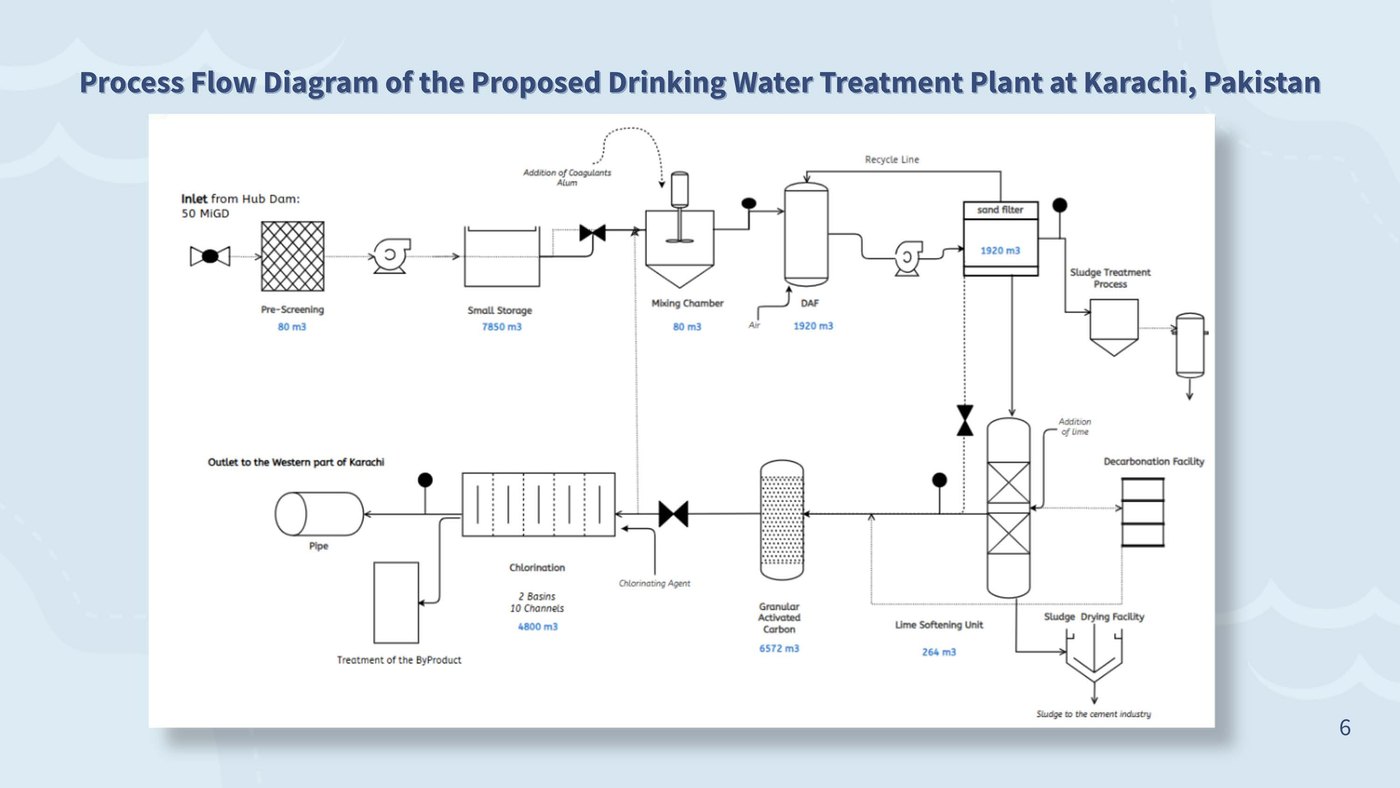
    Academic design estimates, not an operating plant. The team diagram shows an earlier design iteration; the case-study table has the final sizing.
    ExcelProcess designHydraulicsCAPEX / OPEX
    Process flow diagram of the proposed drinking-water treatment plant at Karachi, from intake and screening through flotation, filtration, softening and disinfection to storage.
    Team process-flow diagram of the treatment train. Unit volumes in the diagram are from an earlier design iteration, and its "MiGD" should read US MGD; the table in the case study has the final sizing.
    Full case study: design basis, units, economics

    Context

    Karachi supplies about 650 MGD against 820–1,200 MGD of demand. Karachi water-quality data show hardness up to 2,000 mg/L CaCO₃ and turbidity up to 65 NTU, which the design takes as its basis, so the plant needs softening and strong particle removal, not just disinfection.

    Design basis

    1.5 m intake pipe at 1.24 m/s (Re ≈ 1.4 × 10⁶, 0.10 bar loss over 0.5 km). Alum 70 mg/L, chlorine 5 mg/L, COD 60 mg/L, activated-carbon capacity 600 mg COD/g, 20 min empty-bed contact time, 1% water loss.

    Treatment train and unit sizes

    StepPurposeSize
    Storagebuffer raw water2 × 3,927 m³
    Dissolved-air flotationremove flocs and turbidity12 × 160 m³
    Sand filtrationpolish particles12 units
    Lime softeningreduce hardnesslime 1,423 mg/L
    Activated carbonremove organics4 × 657 m³ (20 min contact)
    Chlorinationdisinfection4,800 m³ · 39.4 kg Cl₂/h

    Economics

    CAPEX $90.0 M plus 5% contingency. In the team's cost breakdown, disinfection (35.5%) and activated carbon (34.2%) are the largest items. Cash-flow analysis gives an IRR of 8%, above the 6–7% hurdle rate.

    Limits

    Academic design estimates, not an operating plant. The team flagged public trust, high utility costs and governance as the main delivery risks.

    Type
    Course case study
    Context
    BME · waste-heat utilisation
    Period
    Dec 2025
    Team
    Individual

    CHP case analysis · heat demand · investment case

    Gas CHP for a London university campus

    Should a London university campus run its own combined heat and power unit, and how big? A course presentation working through a published CHP assessment (Amber et al., 2018).
    Problem
    A CHP unit only pays off when its heat is used, so sizing against the campus load profile decides the case.
    My part
    Individual: load analysis, sizing logic, investment case and price sensitivity, analysed and presented from the published study.
    Result
    215 kWel / 304 kWth option under the winter heat and electrical base loads; the study estimates −395 t CO₂/yr and a payback of 4.5–15 years across price scenarios.
    Limit
    Concept-level: load, CO₂ and savings figures come from the published assessment, not recalculated from scratch.
    Load analysisCHP case analysisPaybackPrice sensitivity
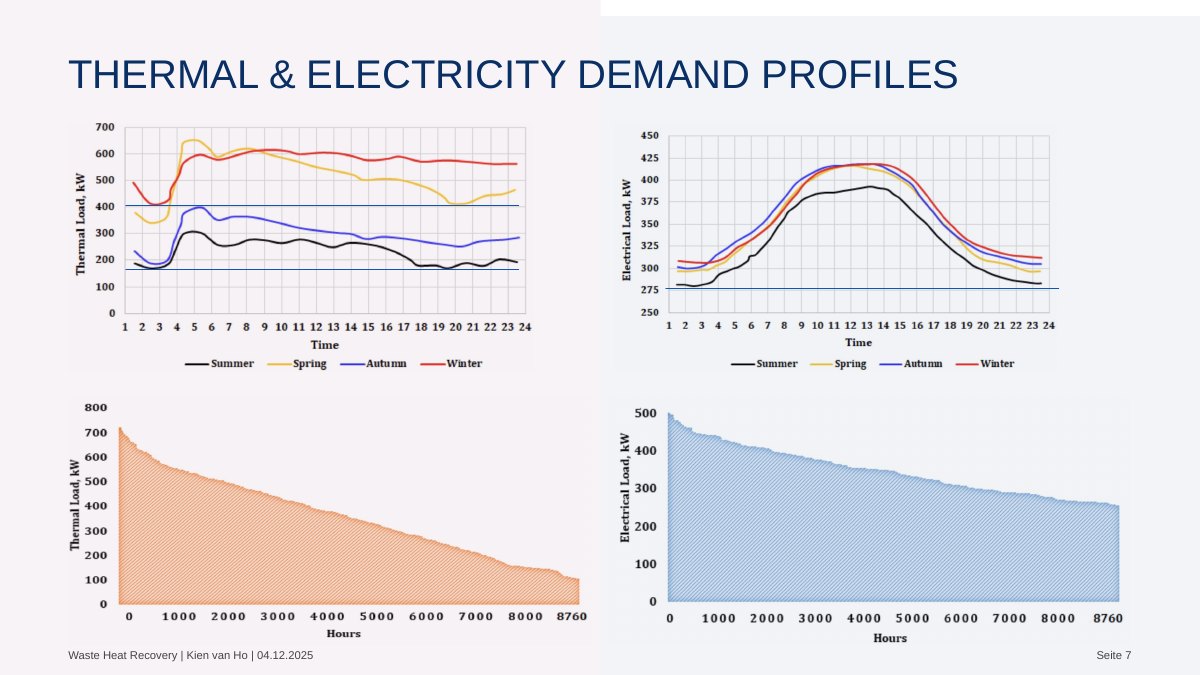
    Seasonal thermal and electricity demand profiles over a day and annual load-duration curves for the campus.
    Seasonal demand profiles and load-duration curves from the published case study (Amber et al., 2018), as used in my presentation.
    Full case study: loads, sizing, finance

    Baseline

    Existing boilers total 4,950 kW (3 × 1,500 + 450 kW). Annual use is about 4.2 GWh of heat and 3 GWh of electricity. Thermal base load is 400 kW in winter and 180 kW in summer; electrical base load is 275 kW.

    Sizing logic in the study

    A CHP only pays off when its heat is used, so the unit sits under the winter heat base load (400 kW) and the electrical base load (275 kW) to run long hours: 215 kW electrical and 304 kW thermal at about 5,000 h/yr. Part-load efficiency ranges from 29–32% electrical and 42–49% thermal. A second option runs 24/7 below the electrical base load to cover 47% of one building's power.

    Investment case

    • CAPEX about £403,000 and net savings about £51,000 a year
    • Simple payback of roughly 8 years at current prices
    • Gas use rises by about half, so savings depend on the electricity it displaces

    Finding

    Useful heat demand and the electricity-to-gas price ratio decide the case. Higher power prices or cheaper gas shorten payback; across the tested prices it ranged from about 4.5 to 15 years.

    Limits. A concept-level course study: the load data, CO₂ and savings figures come from the published assessment, which I analysed and presented rather than recalculated from scratch. Price uncertainty is the main risk. Detailed design and grid connection were outside its scope.
    Type
    Course project
    Context
    BME · energy storage + planning
    Period
    2025
    Team
    Individual

    Vehicle-to-grid · peak demand · scenarios

    Can parked EVs cover Berlin's evening peak?

    A scenario model of Berlin's battery-electric fleet from 2025 to 2030, estimating how much stored energy owners could feed back during the evening peak, by season and participation rate.

    Problem
    Berlin's evening peak needs flexibility; could the growing EV fleet supply a meaningful share of it by 2030?
    My part
    Individual course project: demand, fleet and battery scenario model built in Excel from published planning-area data.
    Result
    7.8–23.4% of summer evening-peak energy in 2030 (5.0–15.0% in winter), depending on how many owners take part.
    Limit
    Optimistic growth and participation; one planning area's profile scaled citywide; battery wear, economics and local grid limits not modelled.
    ExcelScenario analysisEnergy storageDemand profiles
    0% 10% 20% 30% 7.8 5.0 15.6 10.0 23.4 15.0 25% 50% 75% share of owners taking part
    Summer (18–22 h)Winter (16–21 h)
    Share of Berlin's 2030 evening-peak energy that participating BEVs could supply. My calculation.
    Full case study: model, assumptions, limits

    Demand side

    Evening peak plateaus per Berlin planning area (LOR) taken from Straub et al. (2023): 3.5 MW for 4 h in summer and 6 MW for 5 h in winter, scaled to all 448 areas. That gives 6,272 MWh (summer) and 13,440 MWh (winter) of energy in the peak window.

    Supply side

    Available energy E = N · C · SOC · PR · α · η: fleet size N, 60 kWh battery, 30% of charge released, participation 25/50/75%, simultaneity 0.40 (summer) or 0.55 (winter), 88% discharge efficiency. Fleet grows about 55% a year from 34,000 BEVs in 2025.
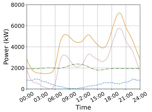
    Daily power profile for one Berlin planning area in winter, with demand peaking above 7,000 kW around 19:00.
    Winter demand (orange), renewable (green) and non-renewable supply (red) for one planning area. Source figure: Straub et al. (2023), used as the demand basis.

    Finding

    In 2025 V2G covers only 0.6–2.6% of the peak. By 2030 fleet growth makes it a meaningful flexibility resource, but how many owners take part and when cars are plugged in matter as much as the number of cars.

    Limits

    One planning area's demand profile scaled to all 448 areas, vehicles spread evenly across the city, fixed simultaneity factors and ideal coordination with the grid. Battery wear, economics, charger roll-out, regulation and local grid limits are not modelled, and the growth and participation rates are optimistic.

    Type
    Internship
    Company
    Mercedes-Benz AG
    Period
    Feb 2023 – Feb 2024
    Team
    Individual (intern)

    Production planning · process data · predictive maintenance

    Industrialising an axial-flux electric motor

    A year in planning and industrialisation for a new axial-flux electric motor: engineering for the new production facilities and data-driven monitoring of a key machine.

    Problem
    A new motor line needed production facilities designed and its critical machines kept reliable.
    My part
    Year-long intern: designed extraction and filtration solutions for the new facilities; analysed critical process parameters of a press.
    Result
    Extraction and filtration concepts for the facilities, and a Power BI dashboard for monitoring and predictive maintenance of the press.
    Limit
    Internal project; documents stay with Mercedes-Benz, so outcomes are described, not shown. Happy to talk through it in an interview.
    Production planningProcess parametersPower BIPredictive maintenance
    Type
    Course project
    Context
    BME · biomass utilisation
    Period
    Nov 2025
    Team
    Individual

    Hydrogen · methanation · energy balance

    Power-to-Gas: hydrogen or synthetic methane?

    Is Power-to-Gas a key technology for the energy transition? Energy and mass balances for both routes, a comparison of electrolyser and methanation technologies, and a real plant case.
    Problem
    Hydrogen or synthetic methane: how much energy survives each route, and at what technology readiness?
    My part
    Individual: energy and mass balances per kWh, electrolyser comparison (SOE, PEM, alkaline), Werlte plant case.
    Result
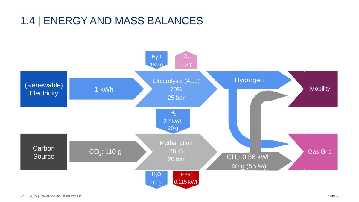
    1 kWh of electricity gives 0.70 kWh of hydrogen (alkaline electrolysis) and about 0.55 kWh of methane after methanation, roughly 55% overall.
    Limit
    Literature values; the real plant runs at 54 ± 3% and is not economic without subsidies.
    Mass & energy balanceElectrolysisMethanationSector coupling
    Energy and mass balance: 1 kWh of renewable electricity through alkaline electrolysis gives 0.7 kWh of hydrogen for mobility; methanation with CO2 gives 0.56 kWh of methane for the gas grid.
    My energy and mass balance per 1 kWh of renewable electricity.
    Full case study: technologies, plant case, verdict

    Electrolyser comparison (literature values)

    TypeEfficiencyTemperatureTRLStack life
    Solid oxide (SOE)81–86%500–1000 °C6–7< 40,000 h
    PEM67–82%50–90 °C8< 20,000 h
    Alkaline (AEL)62–82%60–90 °C9< 90,000 h

    Balance per kWh

    1 kWh of electricity and 189 g of water give 0.7 kWh (20 g) of hydrogen and 168 g of oxygen. Methanation with 110 g of CO₂ gives about 0.55 kWh (40 g) of methane and 0.115 kWh of heat, which is worth recovering.

    Plant case: Werlte e-gas

    6 MW plant producing about 1,300 m³/h of hydrogen and 350 m³/h of synthetic natural gas at 54 ± 3% efficiency, about 4,000 h a year. Electricity is about 70% of operating cost; the plant is not economic without subsidies.

    Verdict

    Hydrogen keeps more of the energy; methanation trades about a fifth of it for compatibility with existing gas grids and storage. Either route is only climate-positive with renewable power and biogenic CO₂.

    Barriers

    High production cost driven by electricity price and utilisation, and unclear legal classification of the gas. Reactor options range from fixed-bed (TRL 9) to three-phase reactors (TRL 5).

    Type
    Course reviews
    Context
    BME smart grids · TU Berlin EV tech
    Period
    2023 and 2025
    Team
    Individual · team of 4

    E-mobility · smart grids · Oct 2025 · individual

    Electric buses in a smart grid

    How e-buses differ from cars for the grid (250–600+ kWh packs vs. 50–120 kWh), which charging set-ups fit which routes, and where smart charging, microgrids and V2G create value. Review of 11 recent sources.

    Battery storage · Jan 2023 · team of 4

    Second life for EV batteries

    What happens to EV batteries below 70–80% capacity: ageing, which chemistries suit reuse, and stationary-storage uses, from a 2.8 MWh Hamburg system built from 100 BMW EVs to a 10 MWh store at Rome airport.

    More detail

    E-bus charging options

    • Depot plug-in: about 50–150 kW, up to 300 kW
    • High-power depot: 150–300 kW and above
    • Pantograph opportunity charging: 300–600 kW and above, in 3–10 minute stops

    Output: a six-phase roll-out roadmap and a value matrix for operators, utilities and cities. V2G with buses has to be weighed against battery wear and warranty limits.

    Second-life findings

    Cycle life differs widely: LTO reaches 3,000–7,000 cycles, NMC and LFP about 2,000. Main barriers are safety, the variety of pack designs, conversion effort and economics. Recycled materials could cut raw-material cost by up to 30%.

    Supporting work

    Course projects, case analyses and literature reviews: smaller in scope than the selected work, set more compactly, with the same case-study detail underneath.

    The energy and process view covers Berlin V2G scenarios, a water treatment plant, the engine digital twin, a campus CHP case analysis and Power-to-Gas.
    The ML side in more depth: the Siemens Energy thesis, a Mercedes-Benz robot energy model and small-data model selection.

    Let's talk

    Looking for an entry-level role in ML, data science or hybrid modelling for the energy transition.

    Looking for an entry-level role in energy-systems or process engineering for the energy transition.

    Kien van Ho · Berlin Sources are named where figures come from published studies or team reports.